Confocal laser scanning microscopy

How-tos

• Switch bit depth to 16 bit data

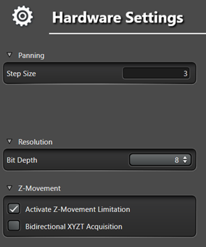
  IMPORTANT: the default bit depth setting will always be 8 bit, not 16 bit. 8 Bit data has a very low quality compared to 16 bit. Always save your data at 16 bit.

  Start of your session

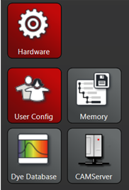
  • In the top bar, on the right of the modules, find and click ‘configuration’

  

  • In the Configuration screen, on the left side, click the button ‘Hardware’

  

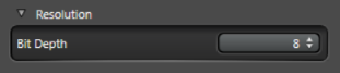
  • The hardware settings windows shows up, in resolution choose ’16 bit’.

  

  • Leave the configuration by clicking ‘Acquire’ in the top of your screen.

• Switch off the lasers at the end of your session

  IMPORTANT: The lasers will not switch off when you close the LAS X software. They may even still be on after you physically switched off the laser switch on the laser rack!

  End of your session

  • Remove your sample
  • Cleaning the microscope
  • In the light path settings near the center of the screen, find the add laser button

  

  • Click the option button right next to it

  

  • The laser rack shows up. Make sure all lasers are OFF before you close the software

  

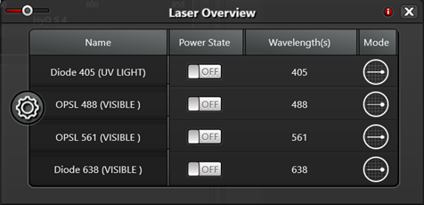
  Only now you can close the software

• Photon counting
  What is photon counting

   Photon counting is a reliable quantitative method for measuring fluorescence. Its main strengths entail:

  • no detector gain
  • no digital-to-analog conversion
  • no intensity corrections
  • minimal noise
  • and the ability to detect with a sensitivity down to a single photon.

   Quantifying fluorescence through photon counting allows for precise measurement of the differences between the lowest possible amount of fluorescence (1 photon) and signals with a few hundreds of photons.

  However, it is crucial to carefully monitor the fluorescence signal and in particular the detector linearity.

  Context

   In photon counting mode, the system electronics are fast enough to be able detect single photons reaching one by one the HyD S detectors photocathode.

   These numbers of photons are then represented in a regular image, whose gray-scale values in this photon counting case corresponds exactly to the number of detected photons. For example, gray-scale value: 15 corresponds to 15 photons.

   Each pixel is filled with photons, much like a basket is filled. The greater the bit depth during this process, the larger the “basket” is, too: a maximum of 4096 photons/pixel can be detected in 12-bit mode, a maximum of 65,356 photons/pixel in 16-bit mode.

  Performing photon counting

  Detectors

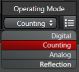
  • Click on the detector(s), and then on the right-end of the detector settings bar you can switch to « Counting » mode for Photon Counting:

  

  • Change the image bit-depth to 12 bits, or 16 bits to be on the safe side. You may detect more than 255 photons in your images (probably), but more than 4096 photons is unlikely. See “Switch Bit depth to 16 bit” in the tab above.

  

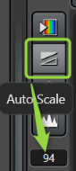
  • Activate the auto-scaling button on the image display. This will help to visualize correctly the image even if just a few photons were collected, specially when working in 12 or 16 bits. The number displayed just below is the number of detected photons in the brightest pixel of the current image, which will be an important value in steps to come.

  

  Detector linearity

   The detection and measurement of the fluorescence signals must be a linear function: a linear relationship between what was emitted by the sample and what ends up in the image.

   To do this correctly, the rule is simple:

  the HyD S detectors are fully linear from 0 to 160 millions detected photons per second (i.e. « 160MHz »). Leica

  Converting this number into a more meaningful time for a confocal system yields: from 0 to 160 detected photons during a dwell time of 1µs ».

   (On the side: that’s much better than any other detector type. For example, a PMT is linear up to 2MHz for example)

   The dwell time is the time spent scanning each pixel of the image. The dwell time will change according to the scan speed, scan format (number of pixels), uni- or bi-directional scan. It can be checked in the software: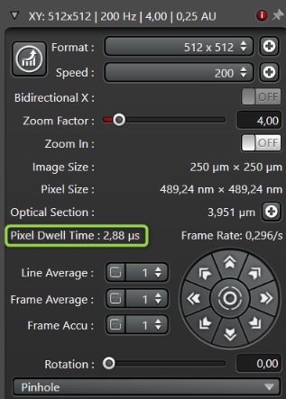

  

  Examples

  A theoretical example

   Assume scanning with precisely a dwell time of 1 µs, adjust the laser excitation power to detect from 0 photons up to a maximum of 160 photons in the brightest pixel of your acquisition, in a single scan. This is easy to check thanks to the autoscaling setting. Any pixel between 0 and 160 photons is perfectly linear and therefore perfectly quantitative relative to the sample.

   Any pixel brighter than 160 photons will show some non-linearity, meaning that the intensity of this pixel is lower than the reality. The non-linearity above 160MHz is very gradual, but it is bad for quantification.

   If this would happpen, only the pixels of the image above 160 photons are off, all the other pixels below 160 photons are fine.

  A realistic example

  On daily basis, in most cases the dwell time will be different than 1µs. In the screen capture below, the dwell time is 2.88µs

  

  How to solve? Multiply your dwell time by 160, yielding the maximum number of photons you should detect on the brightest pixel of your acquisition, in a single scan to remain in the detector linearity regime. Here, 2.88 x 160 = 460 photons maximum. If the dwell time was 4µs: 4×160 = 640 photons maximum, etc.

  Knowing the maximum number of photons that can be detected in a linear way allows now to adjust the laser power accordingly.

  Of course, this is a maximum. There is no problem if the signal is less strong. There is no problem if this maximum cannot be reached – for example because the sample does not emit that many photons – at a reasonable laser excitation. 

  Even more photons?

  What to do if, for example, a minimum of 2000 greyscales/photons is necessary for relevant quantification? Perhaps the laser power cannot be increased due to sample bleaching or charging. In such cases, what measures could be taken to obtain a greater number of photons in the image?

  There are two choices:

  • reduce the scan speed, this will in turn increase the dwell time, which in turn increase the number of detected photons. And with it, the maximum number of photons will increase.
  • apply line or frame accumulations but do not use averaging. Each doubling of the frame doubles the maximum number of photons that can be detected. For example: when a single scan allowed 200 counts, then doing 2 accumulations will allow to have 400 photons in your image. 10 accumulations would allow to have 2000 photons.

  Remarks

  Overall, fluorescent samples are emitting much less photons than one thinks. It’s not unusual to detect only 100 photons from a good sample. An image with 200 photons in the brightest pixel is actually excellent, an image with 2000 photons is insanely good.

  Reaching 12 bits or 4096 detected photons is in many cases possible, but can be time consuming. The scan speed should be reduced and the data accumulation increased to 5 or 10 times, for example. It’s usually not necessary to detect as many photons.

   Reaching 65000 photons to fill a 16 bits dynamic with real photons is near utopic. It may be possible with extremely solid samples (in terms of bleaching) and if a lot of time can be spend (e.g. 20 minutes of more) on a single image scan.
• LIF LOV and autosave

  LIF files are not compatible with auto-saving. They need to be saved during or at the end of the working session. Leica Applications specialist

  TIF files can be autosaved. However, instead of a one tif file per stack, you will get a whole bunch of tif files (one per slice). Quite a bit of regex is needed to reconstruct the data into one file (multiple channels, multiple Z heights, even multiple time points). Leica Applications specialist

  LOF

  The LOF format can also be autosaved, and are compatible with ImageJ/Fiji version 1.54g (since about August 2023).

  Opening LOF files in Fiji

  1. Get FIJI up to date.

  • In Fiji: Help > Update ImageJ… (this will update the ImageJ core of FIJI)

  

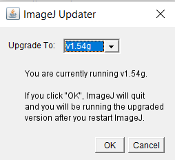
  • Restart Fiji
  • In Fiji: Help > Update… (this will update the Plugins of FIJI, including the Bio-Formats plugin)
  • Restart Fiji

  2. Set the proper settings in LAS X

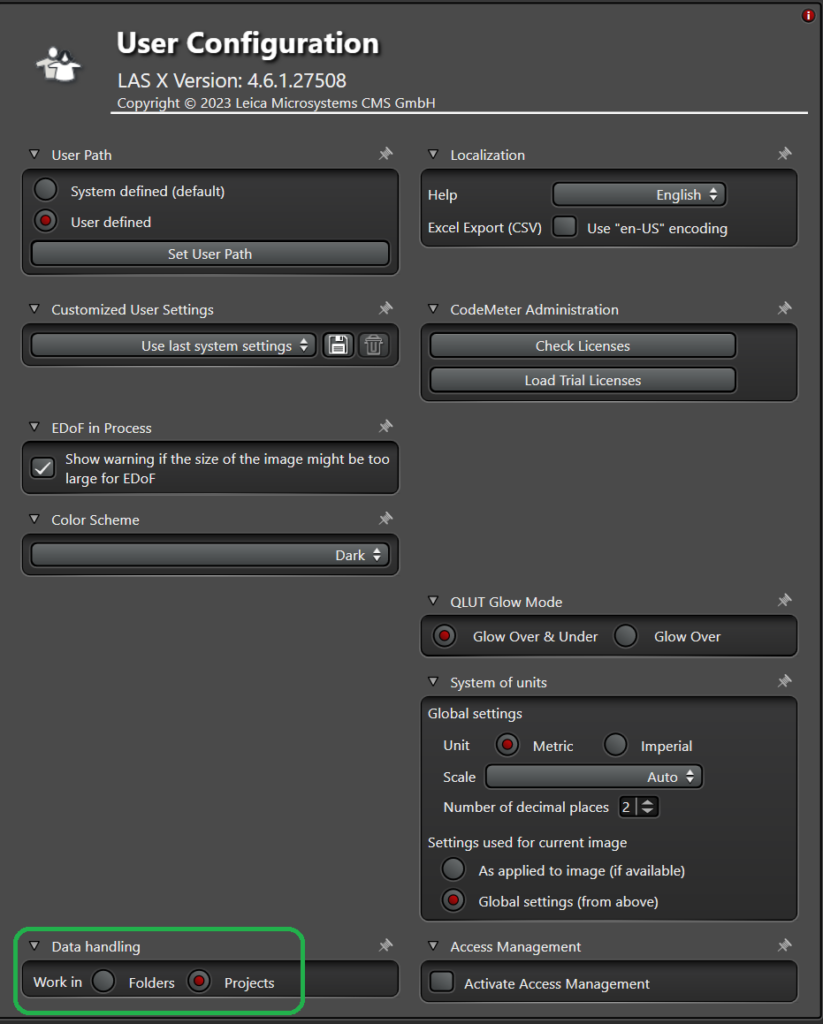
  • In The configuration settings, assure you use “Projects”

  

  

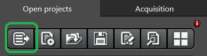
  • Got the the acquire tab

  

  • Into the Projects tree tab

  

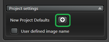
  • At the bottom left, find the Project settings. Choose the + next to New Project Defaults

  

  • Assure that Auto-save is on. As preferred datatype, choose LOF (for TIFF, see above).

  

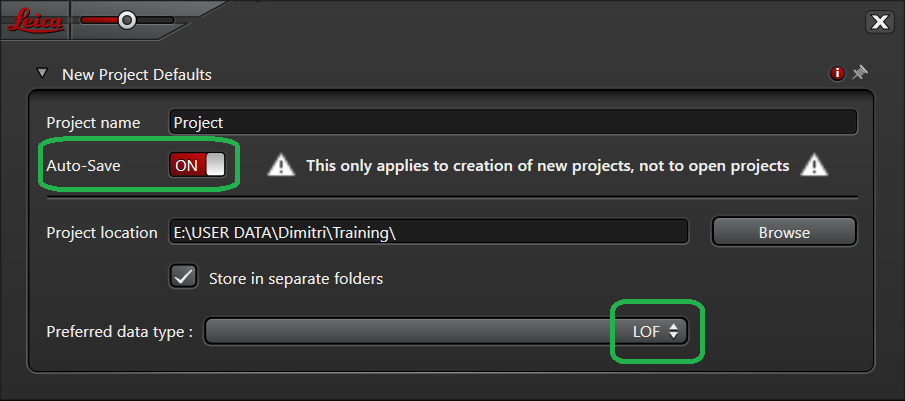
  • Create a bew project and your data will be saved as LOF and XLEF files

  1. Open XLEF and LOF in FIJI

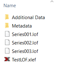
  Your data will appear as:

  • 1 or serveral LOF files
  • one xlef file
  • a Metadata folder
  • an Additional Data folder

  

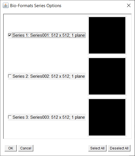
  In FIJI > Plugins > Bio-Formats > Bio-Formats importer

  • Open the XLEF file for a list of all images in the project
  • Open the LOF file to directly open a specific image

  

Advanced training topics

• Advanced tools

  Advanced tools include:

  • Fast live settings
  • Autofocus
  • System optimized resolution
  • Scanning regions of interest (ROI)
  • Resonance scanning
  • Photon counting

   

  Audience: all advanced users

  Time: about 1 hour

• Advanced applications

  Advanced applications assume that you have a thorough understanding of the advanced tools. The applications include:

  • Linear Z compensation
  • Image optimization by dynamic signal enhancement
  • Lambda scanning (spectral imaging)
  • Lambda scanning spectral unmixing (dye separation)
  • the dye database
  • Bleaching / FRET / FRAP
  • Live cell imaging
  • Lightning

   

  Audience: users with specific projects

  Time: about 1/2 day

• Live data mode

  The live data mode allows combining imaging and/or experimental events in real-time.

  • Some examples of the live data mode include:

  • Time Series with different speeds

  • Time Series with a pause

  • Time Series with a recording of a 3D stack

  • Triggered time series

   

  Audience: users with specific projects

  Time: about 1 hour